Tutorial. The Chebyshev interpolation

Spectral methods are the Formula 1 cars of numerical analysis: fast, precise, and, when handled with care, capable of tackling the most challenging computational tracks. In these methods, the solution $u$ is expanded in terms of trial functions:

$$ u(x)\approx\sum_{k=0}^{N-1}\tilde{u}_k\phi_k(x), $$

where the $\tilde{u}_k$ are the expansion coefficients, and the $\phi_k$ are chosen for their mathematical and computational prowess.

But what makes a good trial function? The answer is a blend of convergence, computational efficiency, and ease of differentiation. For non-periodic boundary problems, algebraic polynomials—especially those orthogonal with respect to a weighted $L^2$ scalar product—are the tools of choice. Enter the Chebyshev polynomials.

Chebyshev Polynomials: The Orthogonal Superstars

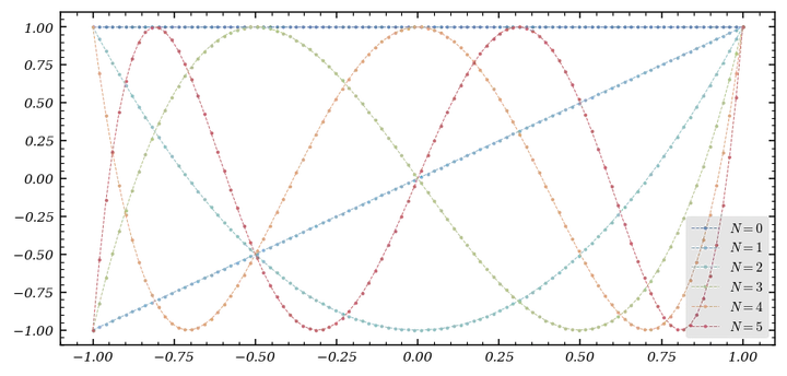
The Chebyshev polynomials of the first kind, $T_k(x)$, are orthogonal on $(-1,1)$ with respect to the weight $w(x)=\frac{1}{\sqrt{1-x^2}}. They satisfy:

$$ T_k(\cos(\theta)) = \cos(k\theta) $$

and can be generated by the recurrence:

$$ \begin{align*} &T_0(x) = 1,\\ &T_1(x) = x,\\ &\forall k\in\mathbb{N}^*,\ T_{k+1}(x) = 2xT_{k}(x)-T_{k-1}(x). \end{align*} $$

The Chebyshev-Gauss-Lobatto (CGL) nodes, $x_j = \cos\left(\frac{\pi j}{N}\right)$, are the extrema of $T_N$ and are the secret to taming the wild oscillations of high-degree polynomial interpolation.

Let’s compute the coefficients of the first $N+1$ Chebyshev polynomials in the canonical basis:

def compute_Chebyshev_coefficients(N : int) -> Callable :
    """
    compute_Chebyshev_coefficients compute the the coefficients in the canonical basis of
    P_N of the N + 1 first Chebyshev polynomial

    Parameters
    ----------
    N : int
        _description_

    Returns
    -------
    Callable
        array of coefficients
    """
    array_coeff = np.zeros(shape = (N+1, N + 1))

    array_coeff[0][0] = 1
    array_coeff[1][1] = 1

    for k in range(2, N + 1) :

        array_coeff[k] = 2 * np.insert(array_coeff[k-1,:-1],0,0) - array_coeff[k-2]

    return array_coeff

And visualize them:

from numpy.polynomial.polynomial import polyval

fig, ax = plt.subplots()
color = color_list(6)
x = np.linspace(-1,1, 100)

for N in range(6):
    ax.plot(x, polyval(x,coeffs[N]), '-o', lw = .5, markersize = 1, linestyle = 'dashed', color = color[N], label = f'$N = {N}$')

ax.legend()

Chebyshev Interpolation: Lagrange Meets Chebyshev

Given a function $u$ on $[-1,1]$, we interpolate it at the CGL points, writing the interpolant in the Chebyshev basis:

$$ I_Nu(x)=\sum_{k=0}^N\tilde{u}_kT_k(x). $$

But how do we compute the coefficients $\tilde{u}_k$? The answer is a beautiful connection to the discrete cosine transform:

$$ \tilde u_k = \frac{2}{N \bar c_k} \sum_{j=0}^{N} u(x_j) \frac{1}{\bar c_j} \cos\left(\frac{k \pi}{N} j\right) $$

where $\bar c_j = 2$ if $j=0$ or $N$, and $1$ otherwise.

With scipy.fft.dct, this becomes:

from scipy import fft
def compute_dct_coeff(N : int, u : Callable) :
    """
    compute_Chebyshev_coeff _summary_

    Parameters
    ----------
    N : int
        _description_
    u : Callable
        _description_
    """
    x = np.cos(np.arange(N+1)/N * np.pi)
    u_ = u(x)
    coeffs = fft.dct(u_,  type = 1, norm = 'forward')
    coeffs[1:-1] = 2 * coeffs[1:-1]

    return coeffs

To evaluate the interpolant at arbitrary points:

def interpolant_chebyshev(set_coefficients : Iterable, set_points : Iterable) :
    """
    interpolant_chebyshev _summary_

    Parameters
    ----------
    set_coefficients : _type_
        _description_
    """
    coeffs_chebyshev = compute_Chebyshev_coefficients(len(set_coefficients))
    poly = 0

    for k in range(len(set_coefficients)) :

        poly +=  polyval(set_points, coeffs_chebyshev[k]) * set_coefficients[k]

    return poly

Let’s see Chebyshev interpolation in action for three functions:

$u(x) = \cos((x + 1)\pi) + \sin(2(x + 1)\pi)$,
$u(x) = \mathbb{1}_{\left[-\frac{1}{2},\frac{1}{2}\right]}(x)$,
$u(x) = \dfrac{1}{1+25x^2}$.

fig, ax = plt.subplots(4,3, figsize = (6,9))
x = np.linspace(-1,1,100)
N = [5, 10, 20, 50]
func = [u_1, u_2, u_3]
color = color_list(2)

for k in range(len(N)):
    for j in range(3) :
        ax[k,j].plot(x,func[j](x), color = color[1], label = '$u$')
        ax[k,j].plot(x, interpolant_chebyshev(compute_dct_coeff(N[k], func[j]), x),'--', color = color[0], label = '$I_N u $')
        CGL = np.cos(np.arange(N[k] + 1)/N[k] * np.pi)
        ax[k,j].scatter(CGL, func[j](CGL), s = 15, fc = (0,0,0,0), ec = 'k',  label = 'CGL')
        ax[k,j].set_xlim(-1.2, 1.2)
        ax[k,j].axvspan(-1.2,-1, color = 'grey', alpha = .4)
        ax[k,j].axvspan(1,1.2, color = 'grey', alpha = .4)
        ax[k,j].text(0, np.mean(func[j](x)), f"$N = {N[k]}$", ha = 'center')
        ax[k,j].legend()

Chebyshev interpolation is spectacular for smooth functions, but for discontinuous ones, the Gibbs phenomenon appears—those pesky oscillations near the jump.

Differentiation in the Chebyshev World

The Chebyshev interpolation derivative is the derivative of the interpolant:

$$ \mathcal{D}_Nu=(I_Nu)' = \sum_{k=0}^N\tilde{u}_k{T_k}'(x). $$

A remarkable formula gives the derivative at $x$:

$$ (I_Nu)'(x) = \frac{1}{\sqrt{1-x^2}}\sum_{k=0}^Nk\tilde{u}_k\sin(k\arccos(x)), $$

and at the endpoints:

$$ (I_Nu)'(1)=\sum_{k=0}^Nk^2\tilde{u}_k,\\ (I_Nu)'(-1)=\sum_{k=0}^N(-1)^{k+1}k^2\tilde{u}_k. $$

To compute the derivative at the nodes:

def der_interpolant(coeff_interpolant, nodes) :
    """
    interpolant_chebyshev _summary_

    Parameters
    ----------
    set_coefficients : _type_
        _description_
    """
    coef = 1/np.sqrt(1 - nodes**2)
    k = np.arange(len(coeff_interpolant))
    interpol = np.empty_like(nodes)

    for j in range(len(nodes)) :

        interpol[j] = np.sum(k * coeff_interpolant * np.sin(k *  np.arccos(nodes[j])))

    return coef * interpol

Let’s compare the true derivatives and their Chebyshev interpolants for several $N$:

fig, ax = plt.subplots(4,3, figsize = (6,9))
x = np.linspace(-.99,1,100)
N = [5, 10, 20, 50]
func = [u_1, u_2, u_3]
funcp =[u_1p, u_2p, u_3p]
color = color_list(2)

for k in range(len(N)):
    for j in range(3) :
        ax[k,j].plot(x,funcp[j](x), color = color[1], label = '$u$')
        CGL = np.cos(np.arange(N[k] + 1)/N[k] * np.pi)
        ax[k,j].scatter(CGL, funcp[j](CGL), s = 15, fc = (0,0,0,0), ec = 'k',  label = 'CGL')
        ax[k,j].plot(x, der_interpolant(compute_dct_coeff(N[k], func[j]), x),'--', color = color[0], label = '$I_N u $')
        ax[k,j].set_xlim(-1.2, 1.2)
        ax[k,j].axvspan(-1.2,-1, color = 'grey', alpha = .4)
        ax[k,j].axvspan(1,1.2, color = 'grey', alpha = .4)
        ax[k,j].legend()

The Runge Phenomenon: When Equidistant Nodes Go Rogue

Interpolating at equidistant nodes can be disastrous for certain functions, like $u(x)=\frac{1}{1 + 25x^2}$. As $N$ increases, the interpolant oscillates wildly near the endpoints—a phenomenon known as the Runge phenomenon.

Let’s see this in action:

from scipy.interpolate import lagrange

fig, axes = plt.subplots(2,2, figsize = (5,4))
x = np.linspace(-1,1,100)
N = [5, 10, 20, 50]
color = color_list(2)

for k, ax in enumerate(axes.flat) :
    points = -1 + 2 * np.arange(N[k] + 1)/N[k]
    ax.plot(x,u_3(x), color = color[1], label = '$u$')
    ax.plot(x, lagrange(points, u_3(points))(x),'--', color = color[0], label = '$I_N u $')
    ax.scatter(points, u_3(points), s = 15, fc = (0,0,0,0), ec = 'k',  label = 'nodes')
    ax.set_xlim(-1.2, 1.2)
    ax.axvspan(-1.2,-1, color = 'grey', alpha = .4)
    ax.axvspan(1,1.2, color = 'grey', alpha = .4)
    ax.text(0, np.mean(u_3(x)), f"$N = {N[k]}$", ha = 'center')
    ax.legend()

As $N$ increases, the interpolant diverges near the endpoints—clearly, equidistant nodes are not the way to go for high-degree polynomial interpolation.

Chebyshev Nodes to the Rescue

Now, let’s interpolate at Chebyshev nodes:

fig, axes = plt.subplots(2,2, figsize = (5,4))
x = np.linspace(-.99,1,100)
N = [5, 10, 20, 50]
color = color_list(2)

for k, ax in enumerate(axes.flat) :
    points = np.cos((2 * np.arange(N[k]) +1) / (2 * (N[k] + 1)) * np.pi)
    ax.plot(x,u_3(x), color = color[1], label = '$u$')
    ax.plot(x, lagrange(points, u_3(points))(x),'--', color = color[0], label = '$I_N u $')
    ax.scatter(points, u_3(points), s = 15, fc = (0,0,0,0), ec = 'k',  label = 'nodes')
    ax.set_xlim(-1.2, 1.2)
    ax.axvspan(-1.2,-1, color = 'grey', alpha = .4)
    ax.axvspan(1,1.2, color = 'grey', alpha = .4)
    ax.text(0, np.mean(u_3(x)), f"$N = {N[k]}$", ha = 'center')
    ax.legend()

With Chebyshev nodes, the interpolation remains stable and accurate even for large $N$. The lesson is clear: for polynomial interpolation, Chebyshev nodes are the gold standard.

Conclusion

Chebyshev interpolation combines mathematical elegance with computational efficiency. By choosing the right nodes and leveraging the power of the discrete cosine transform, we can achieve high-accuracy approximations and derivatives, while avoiding the pitfalls of the Runge phenomenon. For smooth functions, Chebyshev interpolation is a near-perfect tool; for discontinuous ones, beware the Gibbs phenomenon—but even then, it’s often the best you can do. Happy interpolating!