Welcome to the world of collocation spectral methods, where we solve partial differential equations (PDEs) with the speed and elegance of spectral expansions. In this notebook, we’ll tackle an initial-value problem for a linear PDE using two algorithmic approaches: one powered by the fast Fourier transform (FFT), the other by the brute force of differentiation matrices.
We’ll need a few trusty libraries, including fft from scipy for efficient Chebyshev transforms:
import numpy as np
import scipy as scp
from scipy import fft

# To draw matplotlib plots within this notebook.
%matplotlib inline
import matplotlib
import matplotlib.pyplot as plt
from python_code.nord_cmap import *
from typing import Iterable, Callable
Differentiation in Collocation Spectral Methods: FFT vs. Matrix Multiplication
When implementing a collocation spectral method, differentiation at the collocation points can be performed in two ways: via FFTs or by multiplying with a differentiation matrix.
Let’s start with the Fourier interpolation derivative matrix \(D_N\). For an even \(N\), the approximate value of the first derivative of a function \(u\) at the collocation point \(x_j=\frac{2\pi j}{N}\) is given by
where
This matrix is a Toeplitz matrix, which means it’s constant along its diagonals—a property that makes it efficient to store and manipulate.
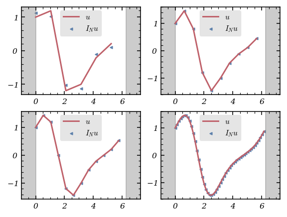
Let’s see how this works in practice for \(u(x)=\exp(\sin(x))\):
from time import time
from fourrier import *

def compute_FIDM(N) :
    j = np.arange(1,N)
    first_column = np.insert(1/2 * (-1) ** j * 1/np.tan(j * np.pi / N),0,0)
    first_row = - first_column
    FIDM = scp.linalg.toeplitz(first_column, first_row)
    return FIDM

def u(x) : return np.exp(np.sin(x))
def u_p(x) : return np.cos(x) * np.exp(np.sin(x))
Let’s compare the accuracy and execution time of matrix-based differentiation and FFT-based differentiation for various \(N\):
fig, axes = plt.subplots(2,2, figsize = (4,3))
color = color_list(2)
N = [6, 10, 12, 50, 80, 100, *[2 ** k for k in range(3, 12)]]

time_mat = []
time_fft = []

error_mat = []
error_fft = []

for k in range(len(N)) :
    collocation = np.arange(N[k]) * 2 * np.pi / N[k]
    t0 = time()
    interp1 = compute_FIDM(N[k]) @ u(collocation)
    time_mat.append(time()- t0)

    t0 = time()
    x = np.linspace(-.99,.99, 100)
    interp2 = der_interpolant(compute_dct_coeff(N[k],u), x)
    time_fft.append(time()- t0)

    error_mat.append(np.max(np.abs(u_p(collocation) - interp1)))
    error_fft.append(np.max(np.abs(u_p(x) - interp2)))

for k,ax in enumerate(axes.flat) :
    collocation = np.arange(N[k]) * 2 * np.pi / N[k]
    interp1 = compute_FIDM(N[k]) @ u(collocation)
    ax.plot(collocation,u_p(collocation), color = color[1], label = '$u$')
    ax.scatter(collocation, interp1,s = 5, marker = '<',color = color[0], label = '$I_N u $')
    ax.set_xlim(-1, 2 * np.pi + 1)
    ax.axvspan(2 * np.pi, 2 * np.pi + 1, color = 'grey', alpha = .4)
    ax.axvspan(-1,0, color = 'grey', alpha = .4)
    ax.legend()
And now, let’s visualize the time and error scaling:
fig, ax = plt.subplots(1,2, figsize = (5,2))

ax[0].scatter(N, time_mat, color = color[0], s = 5, marker = '>', label = 'Matrix')
ax[0].scatter(N, time_fft, color = color[1], s = 5, marker = 'o', label = 'FFT')
ax[0].set_xlabel('N')
ax[0].set_ylabel('time-[s]')
ax[0].set_xscale('log')
ax[0].set_yscale('log')
ax[0].legend()
ax[0].grid(which = 'both', alpha = .4)

ax[1].scatter(N, error_mat, color = color[0], s = 5, marker = '>', label = 'Matrix')
ax[1].scatter(N, error_fft, color = color[1], s = 5, marker = 'o', label = 'FFT')
ax[1].set_xlabel('N')
ax[1].set_ylabel('numerical error')
ax[1].set_xscale('log')
ax[1].set_yscale('log')
ax[1].grid(which = 'both', alpha = .4)
ax[1].legend()
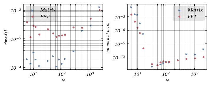
The results are clear: FFT-based differentiation is much faster for large \(N\), while both methods are highly accurate for smooth periodic functions.
For non-periodic functions, Chebyshev interpolation differentiation can also be achieved using a matrix. The Chebyshev differentiation matrix \(D_N\) can be written in closed form:
where \(c_j=2\) if \(j=0\) or \(N\), and \(1\) otherwise, and \(x_j=\cos\left(\frac{\pi j}{N}\right)\).
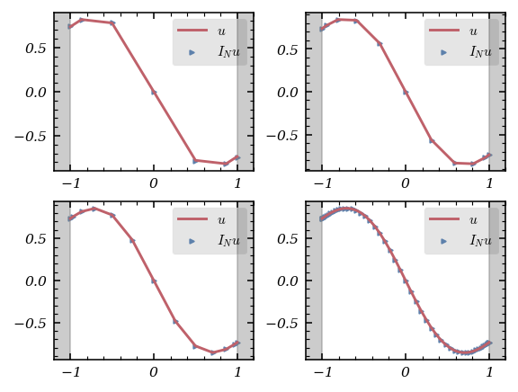
Let’s implement and test this for \(u(x)=\exp(-x^2)\):
def compute_FIDM_np(N) :
    x = np.cos(np.pi * np.arange(N + 1) / N )
    c = np.insert(np.ones(N-1),[0,N-1], [2,2])
    D_N = np.empty(shape = (N+1, N+1))
    for j in range(N + 1) :
        for l in range(N + 1) :
            if j == 0 and l == 0 :
                D_N[j,l] = (2 * N ** 2 + 1) / 6
            if j == N and l == N :
                D_N[j,l] = - (2 * N ** 2 + 1) / 6
            if j == l and j < N and j > 0 :
                D_N[j,l] = - x[j] / (2 * (1 - x[j] ** 2))
            if j != l :
                D_N[j,l] =  c[j]/c[l] * ((-1) ** (j + l)) / (x[j] - x[l])
    return D_N

def u(x) : return np.exp(- x ** 2)
def u_p(x) : return - 2 * x * np.exp(- x ** 2)
And compare matrix and FFT-based differentiation:
fig, axes = plt.subplots(2,2, figsize = (4,3))
color = color_list(2)
N = [6, 10, 12, 50, 80, 100, *[2 ** k for k in range(3, 12)]]

time_mat = []
time_fft = []

error_mat = []
error_fft = []

for k in range(len(N)) :
    collocation = np.cos(np.pi * np.arange(N[k] + 1) / N[k] )
    t0 = time()
    interp1 =compute_FIDM_np(N[k]) @ u(collocation)
    time_mat.append(time()- t0)

    t0 = time()
    x = np.linspace(-.99,.99, 100)
    interp2 = der_interpolant(compute_dct_coeff(N[k],u), x)
    time_fft.append(time()- t0)

    error_mat.append(np.max(np.abs(u_p(collocation) - interp1)))
    error_fft.append(np.max(np.abs(u_p(x) - interp2)))

for k,ax in enumerate(axes.flat) :
    collocation = np.cos(np.pi * np.arange(N[k] + 1) / N[k] )
    ax.plot(collocation,u_p(collocation), color = color[1], label = '$u$')
    ax.scatter(collocation, compute_FIDM_np(N[k]) @ u(collocation), s= 5, marker = '>', color = color[0], label = '$I_N u $')
    ax.set_xlim(-1.2, 1.2)
    ax.axvspan(-1.2, -1, color = 'grey', alpha = .4)
    ax.axvspan(1,1.2, color = 'grey', alpha = .4)
    ax.legend()
fig, ax = plt.subplots(1,2, figsize = (5,2))

ax[0].scatter(N, time_mat, color = color[0], s = 5, marker = '>', label = 'Matrix')
ax[0].scatter(N, time_fft, color = color[1], s = 5, marker = 'o', label = 'FFT')
ax[0].set_xlabel('N')
ax[0].set_ylabel('time-[s]')
ax[0].set_xscale('log')
ax[0].set_yscale('log')
ax[0].legend()
ax[0].grid(which = 'both', alpha = .4)

ax[1].scatter(N, error_mat, color = color[0], s = 5, marker = '>', label = 'Matrix')
ax[1].scatter(N, error_fft, color = color[1], s = 5, marker = 'o', label = 'FFT')
ax[1].set_xlabel('N')
ax[1].set_ylabel('numerical error')
ax[1].set_xscale('log')
ax[1].set_yscale('log')
ax[1].grid(which = 'both', alpha = .4)
ax[1].legend()
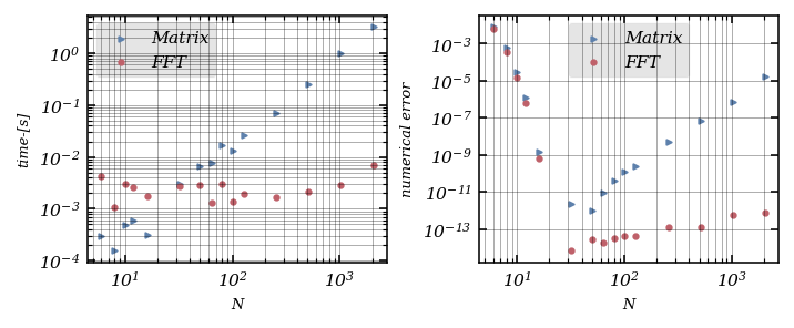
Again, FFT-based differentiation is much faster for large \(N\), but both methods are accurate for smooth functions.
Solving the 2D Wave Equation with a Chebyshev Collocation Spectral Method
Let’s turn up the challenge: we’ll solve the 2D wave equation
with homogeneous Dirichlet boundary conditions and initial data
We’ll use a Chebyshev collocation spectral method in space and a leap-frog scheme in time (the method of lines). The time step \(\Delta t\) must satisfy a CFL-like condition: \(\Delta t\leq C N^{-2}\), with \(C\leq 6.5\).
To compute the second-order Chebyshev interpolation derivative efficiently, we use the discrete Chebyshev coefficients and FFT-based algorithms for \(O(N\log_2 N)\) complexity.
To visualize the solution, we’ll animate the result:
# for animations
matplotlib.rcParams['animation.embed_limit']=2**128
from matplotlib import cm
from mpl_toolkits.mplot3d import Axes3D

from matplotlib import animation
from IPython.display import HTML

# plot the result as an animation
fig,ax=plt.subplots(subplot_kw={"projection": "3d"})
ax.set_xlim((-1.,1))
ax.set_xlabel(r'$x$')
ax.set_ylim((-1.,1.))
ax.set_ylabel(r'$y$')
ax.set_zlim((-1.,1.))
ax.set_zlabel(r'$u(t,x,y)$')

def animate(i,zarray,frame):
    frame[0].remove()
    frame[0]=ax.plot_surface(xx,yy,zarray[i,:,:],rstride=1,cstride=1,cmap=cm.autumn,edgecolor='black')
    ax.set_title(r't='+f'{i*dt:.1f}')

frame=[ax.plot_surface(xx,yy,V[0,:,:],rstride=1,cstride=1,cmap=cm.autumn,edgecolor='black')]

anim=animation.FuncAnimation(fig,animate,nplots,fargs=(V,frame),interval=10)
HTML(anim.to_jshtml())
Second-order Chebyshev interpolation differentiation can also be achieved using a matrix, which can be obtained as the square of the first-order Chebyshev differentiation matrix (at \(O(N^3)\) cost), or directly via the closed-form:
where \(c_j=2\) if \(j=0\) or \(N\), and \(1\) otherwise.
For large-scale problems, FFT-based approaches are preferred for their speed, but matrix-based methods remain valuable for their clarity and directness.
Conclusion
Collocation spectral methods offer a powerful, flexible framework for solving PDEs. Whether you choose the speed of FFTs or the transparency of matrix multiplication, you’ll find these tools indispensable for high-accuracy numerical solutions. And with the right visualization, you can watch your solutions come to life—literally!