Tutorial. Searching for steady states

Welcome to a journey through the fascinating world of dynamical systems, where equations dance, solutions settle, and chaos sometimes reigns. Today, we’ll explore how to hunt for the elusive steady states of a system—those magical points where time stands still and the system finds its balance.

A dynamical system is, at its core, a system described by one or more differential equations that evolves over time. But what happens when the system stops changing? That’s a steady state: a constant solution where the system has found its groove. For a differential equation

u'(t)=f(t,u(t)),

the steady states are found by setting $u'(t)=0$ for all $t$ , so $u(t)=v$ is constant, and solving $f(t,v)=0$ for $v$ .

Let’s get our hands dirty with a concrete example. Consider the autonomous ordinary differential equation:

u'(t)=-(u(t))^3+5\,u(t)+\mu,

where $\mu$ is a real parameter. The steady states are the roots of the polynomial $f_\mu(x)=-x^3+5x+\mu$ . Depending on $\mu$ , there may be one, two, or three real roots—each a possible steady state.

To embark on this adventure, we’ll need a few trusty companions:

import numpy as np

# To draw matplotlib plots within this notebook.
%matplotlib inline
import matplotlib.pyplot as plt
from python_code.nord_cmap import *
from typing import Iterable, Callable

Time-Stepping: Chasing Steady States with Runge-Kutta

Imagine you’re dropped into the landscape of a dynamical system. You pick a starting point and let the system evolve, hoping it’ll settle into a steady state. This is the time-stepping approach: solve the Cauchy problem for various initial conditions and watch where the solutions go as time marches on.

For our cubic system, any solution will eventually converge to a steady state. Why? Because the system’s structure ensures that trajectories are drawn inexorably toward equilibrium—no endless wandering here.

To numerically solve the Cauchy problem, we’ll use the classic fourth-order Runge-Kutta method, whose Butcher’s tableau is a thing of mathematical beauty: $\begin{array}{c|cccc} 0\\ \frac{1}{2}&\frac{1}{2}\\ \frac{1}{2}&0&\frac{1}{2}\\ 1&0&0&1\\ \hline &\frac{1}{6}&\frac{1}{3}&\frac{1}{3}&\frac{1}{6} \end{array}.$

We’ll stop our computation when $|f_\mu(u^{(n)})|\leq\varepsilon$ , with $\varepsilon$ a small tolerance—declaring victory when we’re close enough to a steady state.

Here’s our Runge-Kutta implementation:

def rk4(f : Callable, delta_t : float, init_data : Iterable, tol = .001) -> Iterable:
    """rk4 _summary_

    Parameters
    ----------
    f : Callable
        _description_
    delta_t : float
        _description_
    init_data : Iterable
        _description_
    tol : float, optional
        _description_, by default .001

    Returns
    -------
    Iterable
        _description_
    """
    integrated_data = [init_data]
    h = delta_t
    i = 0

    while np.abs(f(i * delta_t, integrated_data[i])) >= tol :

        i += 1
        time = i*h

        k1 = f(time, integrated_data[i-1])
        k2 = f(time + h/2, integrated_data[i-1] + h * k1/2)
        k3 = f(time + h/2, integrated_data[i-1] + h * k2/2)
        k4 = f(time + h, integrated_data[i-1] + h * k3)

        coeffs = np.array([1/6 * k1, 1/3 * k2, 1/3 * k3, 1/6 * k4])
        Butcheur_sum = np.sum(coeffs, axis = 0)
        integrated_data.append(integrated_data[i-1] + h * Butcheur_sum)

    return np.array(integrated_data)

Let’s see this in action for $\mu=1$ , $u_0=1$ , and a small time step:

mu = 1 ; u0 = 1 ; delta_t = 10 ** (-3)

def f(t, x) : return -x ** 3 + 5 * x + mu

sols = rk4(f, delta_t, u0, tol = .001)

And now, the plot thickens:

fig,ax = plt.subplots()
color = color_list(2)

ax.hlines(sols[-1], 0, len(sols),linestyles='--', lw = .7, color= color[1], label = '$u_\infty$')
ax.plot(sols, lw = 1, color = color[0])
ax.legend(loc = 'center')
ax.set_xlabel('iterations')
ax.set_ylabel('u(t)')

But what if we want to see how the steady states depend on both $\mu$ and the initial value $u_0$ ? Enter the bifurcation diagram—a map of the system’s possible destinies.

mu_array = np.linspace(-10,10, 75)
u0_array = np.linspace(-5,5,75)

Let’s compute the steady states for each combination:

results = np.zeros((75,75))
for k, u0 in enumerate(u0_array) :

    for j, mu in enumerate(mu_array) :

        def f(t, x) : return -x ** 3 + 5 * x + mu
        results[k][j] = rk4(f, delta_t, u0, tol = .001)[-1]

And visualize the landscape:

fig, ax = plt.subplots(figsize = (4,3))
mu_array, u0_array = np.meshgrid(mu_array, u0_array)
img = ax.contourf(mu_array, u0_array, results, cmap = cmap1, levels = 100)
plt.colorbar(img)
ax.set_xlabel('$\mu$')
ax.set_ylabel('$u_0$')

Yet, as beautiful as this diagram is, the time-stepping method can miss some steady states—especially the unstable ones. We need a sharper tool.

Newton-Raphson: The Steady State Detective

When you want to find all the roots—stable or not—there’s nothing quite like the Newton-Raphson method. It’s a classic: start with a guess, and iterate

x^{(k+1)}=x^{(k)}-\frac{f(x^{(k)})}{f'(x^{(k)})}

until you zero in on a solution. It’s fast—quadratically so—when it works, but it can be picky about where you start.

Here’s our implementation:

def newton_raphson(f : Callable, f_prime : Callable, x_0 : float | Iterable, tol = 10 ** (-10), max_iter = 1000) -> Iterable:
    """newton_raphson _summary_

    Parameters
    ----------
    f : Callable
        _description_
    f_prime : Callable
        _description_
    x_0 : float | Iterable
        _description_
    tol : _type_, optional
        _description_, by default 10**(-10)
    max_iter : int, optional
        _description_, by default 1000

    Returns
    -------
    Iterable
        _description_
    """

    x = [x_0]
    i = 0
    while (np.abs(f(x[i])) >= tol) and i <= max_iter:

        x.append(x[i] - f(x[i]) / f_prime(x[i]))
        i += 1
    if i >= max_iter : return np.array([np.infty])

    return np.array(x)

def f_prime(x) : return - 3 * x ** 2 + 5

Let’s watch Newton-Raphson in action, tracking the residuals as it converges (or doesn’t):

x_0 = 1.2

mu_array = np.linspace(-5,5, 10)
fig, ax = plt.subplots(figsize = (3.7,2.5))
color = color_list(len(mu_array))

for i, mu in enumerate(mu_array):

    def f(x) : return -x ** 3 + 5 * x + mu

    ax.loglog(np.abs(f(newton_raphson(f, f_prime,x_0))), linestyle = 'dashed',color = color[i], marker = 'o' ,markersize = 4,lw = .7, label = f'$\mu$ = {mu : .2f}')

ax.legend(loc = 'center left', fontsize = 8)
ax.grid(which = 'both', alpha = .4)

Quadratic convergence is a thing of beauty—but not always guaranteed, especially for tricky values of $\mu$ .

Let’s construct a bifurcation diagram using Newton-Raphson, to see the full spectrum of steady states:

from tqdm import tqdm

mu_array = np.linspace(-10,10, 75)
u0_array = np.linspace(-5,5,75)

results = np.zeros((75,75))

for k, u0 in enumerate(tqdm(u0_array)) :

    for j, mu in enumerate(mu_array) :

        def f(x) : return -x ** 3 + 5 * x + mu
        results[k][j] = newton_raphson(f, f_prime, u0, tol = 10 ** (-10))[-1]

fig, ax = plt.subplots(figsize = (4,3))
mu_array, u0_array = np.meshgrid(mu_array, u0_array)
img = ax.contourf(mu_array, u0_array, results, cmap = cmap1, levels = 500)
plt.colorbar(img)
ax.set_xlabel('$\mu$')
ax.set_ylabel('$u_0$')

Linear Stability: When Steady States Stand Firm (or Wobble)

Steady states are nice, but are they stable? In biology, for example, stability can mean the difference between life and chaos. Let’s look at a model for a repressor protein that regulates its own production—a classic in gene regulation.

The system: $\begin{align*} m'(t)&=\frac{\beta}{1+(p(t))^n}-m(t),\\ r'(t)&=\kappa(m(t)-r(t)),\\ p'(t)&=\gamma(r(t)-p(t)), \end{align*}$

At steady state, all derivatives vanish, and we find a unique solution $(\bar{m},\bar{r},\bar{p})$ with $\bar{m}=\bar{r}=\bar{p}$ and

\bar{m}(1+\bar{m}^n)=\beta.

Linearizing around this steady state, we get a system for the perturbations, with a matrix $A$ whose eigenvalues determine stability: $\begin{pmatrix}\delta m\\\delta r\\\delta p\end{pmatrix}'=\begin{pmatrix}-1&0&-\eta\\\kappa&-\kappa&0\\0&\gamma&-\gamma\end{pmatrix}\begin{pmatrix}\delta m\\\delta r\\\delta p\end{pmatrix},$ where $\eta=\dfrac{n(\bar{m})^n}{1+(\bar{m})^n}$ .

The characteristic polynomial: $\chi_A(X)=X^3+(1+\kappa+\gamma)X^2+(\kappa(1+\gamma)+\gamma)X+(1+\eta)\kappa\gamma.$

Let’s map out the stability in the $\beta$ - $\gamma$ plane:

def linearized_system(kappa : float, eta : float, gamma : float) -> Iterable :
    """linearized_system _summary_

    Parameters
    ----------
    kappa : float
        _description_
    eta : float
        _description_
    gamma : float
        _description_

    Returns
    -------
    Iterable
        _description_
    """
    A = np.array([[- 1 ,   0  , - eta],
                  [kappa, -kappa, 0],
                  [0, gamma, -gamma]])

    return A

Beta = np.logspace(0,4,200) ; n = 10 ; kappa = 1 ; Gamma = np.logspace(-2,2,200)

results = np.zeros((200,200))
for k, beta in enumerate(tqdm(Beta, desc= 'Computing mARN concentration steady state and eighenvalues of the system')) :

    for j, gamma in enumerate(Gamma) :


        def equation_m(x) : return x * (x ** n  + 1) - beta
        def equation_m_prime(x) : return 1 + (n+1) * x ** n

        m_ = newton_raphson(equation_m, equation_m_prime, 0, tol = 10 ** (-8))[-1]
        eta = (n * m_ ** n) / (1 + m_ ** n )

        A = linearized_system(kappa, eta, gamma)
        eigh_vals = np.linalg.eigvals(A)

        if (np.real(eigh_vals) <= 0).all() :
            results[k][j] = 1

        else : results[k][j] = 0

fig, ax = plt.subplots(figsize = (4,3))
Beta_plot, Gamma_plot = np.meshgrid(Beta, Gamma)
img = ax.pcolormesh(Beta_plot, Gamma_plot, results, cmap = cmap1.resampled(2))
ax.set_xlabel(r'$\beta$')
ax.set_ylabel(r'$\gamma$')

ax.set_xscale('log')
ax.set_yscale('log')
plt.colorbar(img, label = 'Stability', drawedges = True, ticks = [0,1   ])

ax.grid(which = 'both', alpha = .5)

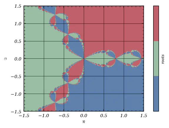
Newton Fractals: The Wild Side of Root-Finding

Let’s end our journey with a trip to the complex plane, where the Newton-Raphson method reveals its fractal soul. Consider $f(z)=z^3-1$ , whose roots are the cube roots of unity. What happens if we start Newton-Raphson from every point in a grid over the complex plane?

Here’s a vectorized Newton-Raphson for the task:

def newton_raphson_vectorize(f : Callable, f_prime : Callable, map_0 : Iterable, tol = 10 ** (-10), max_iter = 300) :
    """newton_raphson_vectorize _summary_

    Parameters
    ----------
    f : Callable
        _description_
    f_prime : Callable
        _description_
    map_0 : Iterable
        _description_
    tol : _type_, optional
        _description_, by default 10**(-10)
    max_iter : int, optional
        _description_, by default 300

    Returns
    -------
    _type_
        _description_
    """
    map = np.copy(map_0)
    i = 0

    while (np.abs(f(map)) >= tol).any() and i <= max_iter: # assume the number of iter is small enough to allow additionnal calculation for valid point

        map -= f(map) / f_prime(map)
        i += 1

    if i > max_iter : map[np.abs(f(map)) >= tol] = np.infty

    return map

Set up the grid and functions:

Re = np.linspace(-1.5, 1.5, 2000) ; Im =  np.linspace(-1.5j, 1.5j, 2000)

Re, Im = np.meshgrid(Re, Im)

def f(z) : return z ** 3 + 1

def f_prime(z) : return 3 * z ** 2

map = newton_raphson_vectorize(f, f_prime, Re + Im)

And behold the Newton fractal:

fig, ax = plt.subplots(figsize = (4,3))

img = ax.pcolormesh(Re, Im.imag, map.imag, cmap = cmap1.resampled(3))

plt.colorbar(img, ticks = [], label = 'roots')
ax.set_xlabel('$\Re$')
ax.set_ylabel('$\Im$')
ax.grid()

The boundaries between basins of attraction are infinitely intricate—proof that even simple equations can hide wild complexity.

For a more pedagogical approach, let’s recast the problem in terms of real variables and use the Jacobian:

Re = np.linspace(-1.5, 1.5, 500) ; Im =  np.linspace(-1.5, 1.5, 500)

Re, Im = np.meshgrid(Re, Im)

def F(x,y) : return np.array([x ** 3 - 3 * y ** 2 * x - 1,
                              3 * x ** 2 * y - y ** 3])

def D_F(x,y) : return np.array([[3 * x ** 2 - 3 * y ** 2, - 6 * y * x],
                                [6 * y * x, 3 * x ** 2 - 3 * y ** 2]])

from scipy import linalg

def newton_raphson_pedagogical(map_0x, map_0y, tol = 10 ** (-10), max_iter = 300) :

    map =  np.empty_like(map_0x, dtype = complex)

    n, p = map_0x.shape

    for k in tqdm(range(n)) :

        for j in range(p) :

            x = map_0x[k,j] ; y = map_0y[k,j]
            i = 0

            while (np.abs(F(x,y)) >= tol).all() and i <= max_iter :

                F_ = F(x,y) ; D_ = D_F(x,y)

                x,y  = np.array([x,y]) - linalg.inv(D_) @ F_

                i += 1

            if i > max_iter : x,y = np.infty, np.infty

            map[k,j] = complex(x,y)

    return map

map = newton_raphson_pedagogical(Re, Im)

fig, ax = plt.subplots(figsize = (4,3))

img = ax.pcolormesh(Re, Im, map.imag, cmap = cmap1.resampled(3))

plt.colorbar(img, ticks = [], label = 'roots')
ax.set_xlabel('$\Re$')
ax.set_ylabel('$\Im$')
ax.grid()

And there you have it: from steady states to fractals, the world of dynamical systems is as rich and surprising as any landscape in science. Whether you’re seeking stability or courting chaos, the tools of numerical analysis are your compass and map. Happy exploring!